Depression Classification using Textual Data

Introduction

In the realm of machine learning, the ability to detect and classify mental health related issues from textual data has significant implications for public health and well being. In this blog post, I will walk you through the process of building a multi-class logistic regression model for depression classification using textual data.

Problem Statement

The goal is to develop a model that can accurately classify text into three categories: "Yes" (indicating the presence of depression), "No" (indicating the absence of depression), and "Neutral" (for a neutral state). This task is essential for providing early insights into individuals' mental health and facilitating timely intervention.

Data Exploration and Preprocessing

The first step is to explore and understand the dataset. In our case, we have this dataset containing text content and corresponding labels. The labels will later be encoded into numerical values for simplicity.

import pandas as pd
import re
import spacy
import matplotlib.pyplot as plt
import seaborn as sns
from sklearn.linear_model import LogisticRegression
from sklearn.metrics import classification_report, accuracy_score, confusion_matrix
import joblib
from sklearn.feature_extraction.text import TfidfVectorizer
from sklearn.model_selection import train_test_split
import numpy as np


# now I load the spaCy English model
nlp = spacy.load('en_core_web_sm')



# Load the CSV dataset into a Pandas DataFrame
data = pd.read_csv("/content/100_line_depression_data.csv")

# Display the first 5 rows of my dataset
data.head()

This code block above is a script for natural language processing (NLP) and machine learning using the spaCy library, pandas, and scikit-learn. The necessary libraries, including pandas for data manipulation, re for regular expressions, spacy for NLP tasks, and matplotlib/seaborn for data visualization, are imported. Additionally, logistic regression is imported from scikit-learn for classification, and TfidfVectorizer is used for text feature extraction. The spaCy English model is loaded for NLP tasks. The dataset is loaded into a Pandas DataFrame named 'data.' The first five rows of the dataset are displayed for initial exploration.

# I am defining a small function to handle my text cleaning and preprocessing steps
def preprocess_text(text):
    # Remove special characters, numbers, and extra spaces
    text = re.sub(r'[^a-zA-Z\s]', '', text)
    text = re.sub(r'\s+', ' ', text).strip()


    # Tokenization using spaCy
    doc = nlp(text)
    tokens = [token.text for token in doc]

    # Join the tokens back into a cleaned text
    cleaned_text = ' '.join(tokens)

    return cleaned_text

# Apply the preprocessing function to the 'Text Content' column
data['Cleaned Content'] = data['Text Content'].apply(preprocess_text)

# Display by comparing both cleaned and preprocessed text
data[['Text Content', 'Cleaned Content']].head()

Moving to the next stage, the code defines a concise Python function, preprocess_text, for text cleaning and preprocessing. It efficiently removes special characters, numbers, and extra spaces using regular expressions and employs spaCy for tokenization. Applied to the 'Text Content' column in the dataset, this function creates a new 'Cleaned Content' column. The final code snippet displays the initial and cleaned text content for the first five rows, streamlining the text data for further analysis by eliminating noise and ensuring a standardized format.

# Define a mapping for the Integer encoding process
indicator_mapping = {'Yes': 1, 'No': 0, 'Neutral': 2}

# Applying the the Integer encoding to the 'Depression Indicator' column
data['Encoded Depression Indicator'] = data['Depression Indicator'].map(indicator_mapping)

# Display the updated DataFrame with the encoded depression indicator column
data[['Depression Indicator', 'Encoded Depression Indicator']].head()

In this step, categorical values in the 'Depression Indicator' column are encoded into integers using a mapping defined in the 'indicator_mapping' dictionary. The Pandas map function facilitates this encoding, resulting in a new column named 'Encoded Depression Indicator.' The updated DataFrame displays both the original categorical values and their corresponding integer-encoded representations. This transformation is a common preprocessing practice in machine learning, essential for preparing categorical data for algorithmic training and prediction.

data.isnull().sum()

Progressing further,data.isnull().sum() is used to identify the number of missing values in each column of the 'data' DataFrame. The isnull() method checks each element in the DataFrame and returns a boolean DataFrame of the same shape, where True indicates a missing value (NaN), and False indicates a non-missing value. The sum() function is then applied to this boolean DataFrame, resulting in a series where each value represents the sum of missing values in the corresponding column. its output provides a quick overview of the missing data distribution, allowing for further analysis and potential handling of missing values in the dataset.

data.describe()

Advancing to the following step,data.describe() generates descriptive statistics for the numeric columns in the 'data' DataFrame. The describe() function provides key statistical measures such as count, mean, standard deviation, minimum, 25th percentile (Q1), median (50th percentile or Q2), 75th percentile (Q3), and maximum for each numeric column. These statistics offer insights into the central tendency, dispersion, and shape of the distribution of numerical data. By running this code, you obtain a summary of the dataset's numeric features, facilitating an initial understanding of the distribution and scale of the numerical variables.

Exploratory Data Analysis (EDA)

This is a crucial initial step in our data analysis where the primary goal is to understand and summarize the main characteristics of a dataset. EDA involves the use of statistical and visualization techniques to gain insights into the data, identify patterns, detect outliers, and inform subsequent modeling or decision-making processes.

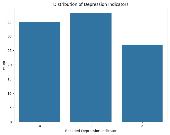
plt.figure(figsize=(8, 6))
sns.countplot(x='Encoded Depression Indicator', data=data)
plt.title('Distribution of Depression Indicators')
plt.show()

The code snippet above uses the matplotlib and seaborn libraries to create a count plot, visualizing the distribution of the 'Encoded Depression Indicator' column in the 'data' DataFrame.This visualization provides a clear representation of the distribution of depression indicators in the dataset, helping to understand the balance or imbalance between different indicator categories.

data['Text Length'] = data['Cleaned Content'].apply(len)
plt.figure(figsize=(8, 6))
sns.histplot(data['Text Length'], bins=30, kde=True)
plt.title('Distribution of Text Lengths')
plt.xlabel('Text Length')
plt.show()

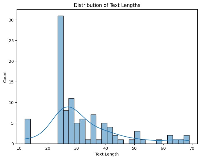
Now we calculate the length of each cleaned text entry in the 'Cleaned Content' column, creating a new 'Text Length' column. A histogram is then generated to visualize the distribution of text lengths. The plot, with a kernel density estimate and 30 bins, offers a concise overview of how text lengths are distributed in the dataset, providing insights into the range and concentration of text lengths for further analysis.

plt.figure(figsize=(10, 6))
sns.boxplot(x='Encoded Depression Indicator', y='Text Length', data=data)
plt.title('Distribution of Text Lengths by Depression Indicator')
plt.show()

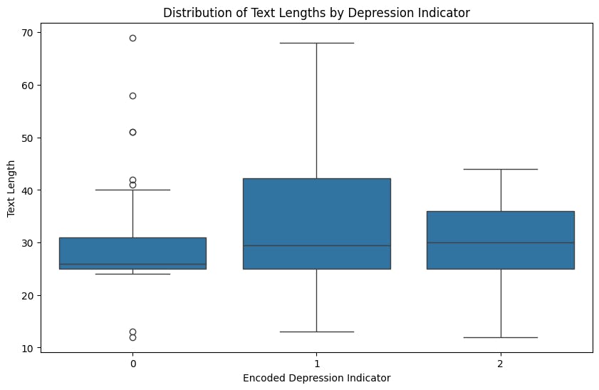
The code generates a boxplot illustrating the distribution of text lengths based on the encoded depression indicators. This visualization provides a concise summary of the central tendency, spread, and potential outliers in text lengths for each depression indicator category (0, 1, 2). The plot facilitates a quick comparison of text length distributions across different depression indicators, aiding in understanding any potential patterns or variations.

columns_to_drop = ["Entry ID", "Text Content", "Depression Indicator", "Source", "Text Length"]
data = data.drop(columns=columns_to_drop)

Now this code removes specified columns ("Entry ID," "Text Content," "Depression Indicator," "Source," and "Text Length") from the 'data' DataFrame, creating a streamlined version of the dataset with only the relevant features for subsequent analysis or modeling.

Feature Engineering: TF-IDF Vectorization

To transform the textual data into numerical features, we employed TF-IDF vectorization. This technique assigns importance scores to words based on their frequency in a document and their rarity across the entire corpus.

# Split the data into training and testing sets
X_train, X_test, y_train, y_test = train_test_split(data['Cleaned Content'], data['Encoded Depression Indicator'], test_size=0.2, random_state=42)

# Initialize the TF-IDF vectorizer
tfidf_vectorizer = TfidfVectorizer(max_features=5000, stop_words='english')

# Fit and transform the training data
X_train_tfidf = tfidf_vectorizer.fit_transform(X_train)

# Transform the testing data
X_test_tfidf = tfidf_vectorizer.transform(X_test)

# Display the shape of the TF-IDF matrices
print("TF-IDF Matrix Shape (Training):", X_train_tfidf.shape)
print("TF-IDF Matrix Shape (Testing):", X_test_tfidf.shape)

Entering the next segment, we divide the dataset into training and testing sets, using 'Cleaned Content' as the input feature and 'Encoded Depression Indicator' as the target variable. It employs a TF-IDF vectorizer with a maximum of 5000 features and removes English stop words. The training data is fitted and transformed, and the testing data is transformed accordingly. The code concludes by displaying the shapes of the resulting TF-IDF matrices for both training and testing sets, offering insights into the dimensions of the feature matrices prepared for subsequent machine learning tasks.

Model Development: Multi-Class Logistic Regression

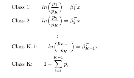
For this classification task, we chose a multi-class logistic regression model due to its simplicity and effectiveness in text classification.

# let's goooooo, first , lemme initialize the Logistic Regression model for multi-class classification
logistic_regression_model = LogisticRegression(random_state=42, max_iter=500, multi_class='ovr')

# Second lemme train the model on the TF-IDF features and integer-encoded target labels
logistic_regression_model.fit(X_train_tfidf, y_train)

# Third lemme do the predictions on the testing set
y_pred = logistic_regression_model.predict(X_test_tfidf)

# Fourth I wanna evaluate the model
accuracy = accuracy_score(y_test, y_pred)
classification_rep = classification_report(y_test, y_pred)


# and then saving the trained TF-IDF vectorizer and Multi-class Logistic Regression model so that I can be able to use them later
joblib.dump(tfidf_vectorizer, 'tfidf_vectorizer.pkl')
joblib.dump(logistic_regression_model, 'logistic_regression_model.pkl')

# now showing the model evaluation metrics
print("Accuracy (Multi-Class Logistic Regression):", accuracy)
print("\nClassification Report (Multi-Class Logistic Regression):\n", classification_rep)

The code initializes, trains, and evaluates a Logistic Regression model for multi-class classification. After setting up the model with specific parameters, it is trained on TF-IDF features and integer-encoded target labels. Predictions are made on the testing set, and model performance is assessed through accuracy and a classification report. The trained TF-IDF vectorizer and Logistic Regression model are saved for future use. The code concludes by displaying the accuracy and classification report metrics, providing insights into the model's effectiveness in multi-class classification.

Training and Evaluation

X_test_tfidf = tfidf_vectorizer.transform(X_test)

# Predictions on the testing set
y_pred = logistic_regression_model.predict(X_test_tfidf)

# Calculate the confusion matrix
cm = confusion_matrix(y_test, y_pred)

# Plot the confusion matrix using seaborn
labels = ['No', 'Neutral', 'Yes']
sns.heatmap(cm, annot=True, fmt='d', cmap='Blues', xticklabels=labels, yticklabels=labels)
plt.title('Confusion Matrix')
plt.xlabel('Predicted')
plt.ylabel('Actual')
plt.show()

We are now transforming the testing set using TF-IDF, predicts outcomes with a Logistic Regression model, calculates the confusion matrix, and plots it using seaborn. The confusion matrix visually represents the model's performance, indicating true positives, true negatives, false positives, and false negatives. The heatmap provides an annotated overview of the predictions, helping to evaluate the model's classification accuracy.

Model Testing

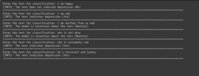
This code snippet constitutes the last part of the project. It loads a pre-trained TF-IDF vectorizer and Logistic Regression model. The provided function, classify_depression(), enables users to input new sentences for model testing. The user input is transformed using the TF-IDF vectorizer, and the model predicts whether the text indicates depression ('Yes'), does not indicate depression ('No'), or if the model is uncertain ('Neutral'). The loop allows users to test the model with multiple inputs. This custom function serves as a practical tool for users to interactively assess the model's predictions based on their input sentences.

# Load the trained TF-IDF vectorizer
tfidf_vectorizer = joblib.load('tfidf_vectorizer.pkl')

# Load the trained Logistic Regression model
logistic_regression_model = joblib.load('logistic_regression_model.pkl')

# Function to classify depression based on user input
def classify_depression():
    # Get user input
    user_input = input("Enter the text for classification: ")

    # Transform the user input using the TF-IDF vectorizer
    user_input_tfidf = tfidf_vectorizer.transform([user_input])

    # Predict using the trained model
    prediction = logistic_regression_model.predict(user_input_tfidf)

    # Display the prediction
    if prediction[0] == 1:
        print("[INFO]: The text indicates depression.(Yes)")
        print("====================================================================================================================")
    elif prediction[0] == 0:
        print("[INFO]: The text does not indicate depression.(No)")
        print("====================================================================================================================")

    else:
        print("[INFO]: The model is uncertain about the text.(Neutral)")
        print("====================================================================================================================")


# Call the function to classify user input
my_testing_time = 5
i = 0
while i <= my_testing_time :
  classify_depression()
  i += 1

Conclusion and Recommendations

In conclusion, the multi-class logistic regression model, coupled with TF-IDF vectorization, provides a solid foundation for depression classification based on textual data. However, the journey doesn't end here. Further exploration could involve experimenting with more advanced models, fine-tuning hyperparameters, and exploring additional text preprocessing techniques.

Building models for mental health classification is a delicate yet crucial task. As the field of machine learning continues to evolve, so does our ability to leverage technology for the betterment of mental health diagnostics and interventions.

Thank you for joining me on this journey of leveraging machine learning for mental health awareness and classification. If you have any questions or suggestions, feel free to reach out.

Happy coding and mental health advocacy!